Bayesian bootstrap posterior sampler for the CDF

Compute one Monte Carlo draw from the Bayesian bootstrap (BB) posterior distribution of the cumulative distribution function (CDF).

Usage

bb(y)

Arguments

y

the data from which to infer the CDF (preferably sorted)

Value

a function that can evaluate the sampled CDF at any argument(s)

Details

Assuming the data y are iid from an unknown distribution, the Bayesian bootstrap (BB) is a nonparametric model for this distribution. The BB is a limiting case of a Dirichlet process prior (without any hyperparameters) that admits direct Monte Carlo (not MCMC) sampling. This function computes one draw from the BB posterior distribution for the CDF Fy.

Note

This code is inspired by ggdist::weighted_ecdf.

Examples

# Simulate data:
y = rnorm(n = 100)

# One draw from the BB posterior:
Fy = bb(y)

class(Fy) # this is a function
#> [1] "function"
#' Fy(0) # some example use (for this one draw)
Fy(c(.5, 1.2))
#> [1] 0.6692355 0.8765828

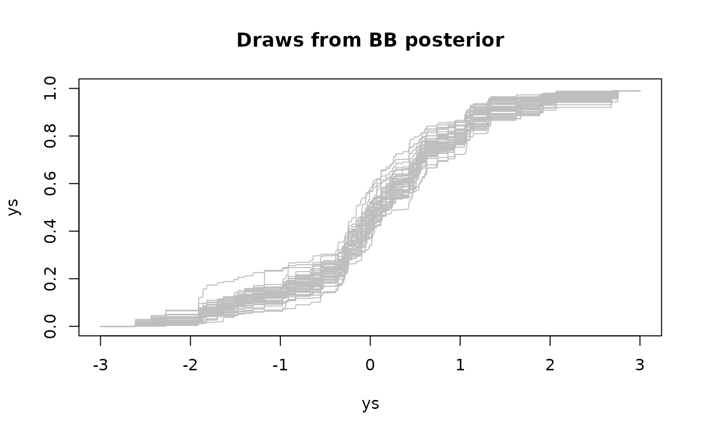
# Plot several draws from the BB posterior distribution:
ys = seq(-3, 3, length.out=1000)
plot(ys, ys, type='n', ylim = c(0,1), main = 'Draws from BB posterior')
temp = sapply(1:50, function(...) lines(ys, bb(y)(ys), col='gray'))