Introduction to SeBR

Background: semiparametric regression via data transformations

Data transformations are a useful companion for parametric regression models. A well-chosen or learned transformation can greatly enhance the applicability of a given model, especially for data with irregular marginal features (e.g., multimodality, skewness) or various data domains (e.g., real-valued, positive, or compactly-supported data).

We are interested in providing fully Bayesian inference for semiparametric regression models that incorporate (1) an unknown data transformation and (2) a useful parametric regression model. For paired data $\{x_i, y_i\}_{i=1}^n$ with $x_i \in \mathbb{R}^p$ and $y \in \mathcal{Y} \subseteq \mathbb{R}$ , consider the following class of models: $g(y_i) = z_i$ $z_i = f_\theta(x_i) + \sigma \epsilon_i$ Here, $g$ is a (monotone increasing) data transformation to be learned, $f_\theta$ is an unknown regression function parametrized by $\theta$ , and $\epsilon_i$ are independent errors. Location and scale restrictions (e.g., $f_\theta(0) = 0$ and $\sigma =1$ ) are usually applied for identifiability.

Examples. We focus on the following important special cases:

The linear model is a natural starting point: $z_i = x_i'\theta + \sigma\epsilon_i, \quad \epsilon_i \stackrel{iid}{\sim} N(0, 1)$ The transformation $g$ broadens the applicability of this useful class of models, including for positive or compactly-supported data (see below).
The quantile regression model replaces the Gaussian assumption in the linear model with an asymmetric Laplace distribution (ALD) $z_i = x_i'\theta + \sigma\epsilon_i, \quad \epsilon_i \stackrel{iid}{\sim} ALD(\tau)$ to target the $\tau$ th quantile of $z$ at $x$ , or equivalently, the $g^{-1}(\tau)$ th quantile of $y$ at $x$ . The ALD is quite often a very poor model for real data, especially when $\tau$ is near zero or one. The transformation $g$ offers a pathway to significantly improve the model adequacy, while still targeting the desired quantile of the data.
The Gaussian process (GP) model generalizes the linear model to include a nonparametric regression function, $z_i = f_\theta(x_i) + \sigma \epsilon_i, \quad \epsilon_i \stackrel{iid}{\sim} N(0, 1)$ where $f_\theta$ is a GP and $\theta$ parameterizes the mean and covariance functions. Although GPs offer substantial flexibility for the regression function $f_\theta$ , the default approach (without a transformation) may be inadequate when $y$ has irregular marginal features or a restricted domain (e.g., positive or compact).

Challenges: The goal is to provide fully Bayesian posterior inference for the unknowns $(g, \theta)$ and posterior predictive inference for future/unobserved data $\tilde y(x)$ . We prefer a model and algorithm that offer both (i) flexible modeling of $g$ and (ii) efficient posterior and predictive computations.

Innovations: Our approach (https://doi.org/10.1080/01621459.2024.2395586) specifies a nonparametric model for $g$ , yet also provides Monte Carlo (not MCMC) sampling for the posterior and predictive distributions. As a result, we control the approximation accuracy via the number of simulations, but do not require the lengthy runs, burn-in periods, convergence diagnostics, or inefficiency factors that accompany MCMC. The Monte Carlo sampling is typically quite fast.

Using `SeBR`

The R package SeBR is installed and loaded as follows:

# install.packages("devtools")
# devtools::install_github("drkowal/SeBR")
library(SeBR)

The main functions in SeBR are:

sblm(): Monte Carlo sampling for posterior and predictive inference with the semiparametric Bayesian linear model;
sbsm(): Monte Carlo sampling for posterior and predictive inference with the semiparametric Bayesian spline model, which replaces the linear model with a spline for nonlinear modeling of $x \in \mathbb{R}$ ;
sbqr(): blocked Gibbs sampling for posterior and predictive inference with the semiparametric Bayesian quantile regression; and
sbgp(): Monte Carlo sampling for predictive inference with the semiparametric Bayesian Gaussian process model.

Each function returns a point estimate of $\theta$ (coefficients), point predictions at some specified testing points (fitted.values), posterior samples of the transformation $g$ (post_g), and posterior predictive samples of $\tilde y(x)$ at the testing points (post_ypred), as well as other function-specific quantities (e.g., posterior draws of $\theta$ , post_theta). The calls coef() and fitted() extract the point estimates and point predictions, respectively.

Note: The package also includes Box-Cox variants of these functions, i.e., restricting $g$ to the (signed) Box-Cox parametric family $g(t; \lambda) = \{\mbox{sign}(t) \vert t \vert^\lambda - 1\}/\lambda$ with known or unknown $\lambda$ . The parametric transformation is less flexible, especially for irregular marginals or restricted domains, and requires MCMC sampling. These functions (e.g., blm_bc(), etc.) are primarily for benchmarking.

Semiparametric Bayesian linear models with `sblm`

We simulate data from a transformed linear model:

set.seed(123) # for reproducibility

# Simulate data from a transformed linear model:
dat = simulate_tlm(n = 200,  # number of observations
                   p = 10,   # number of covariates 
                   g_type = 'step' # type of transformation (here, positive data)
                   )
# Training data:
y = dat$y; X = dat$X 

# Testing data:
y_test = dat$y_test; X_test = dat$X_test

sblm() quickly produces Monte Carlo samples of $(\theta, g, \tilde y(X_{test}))$ under the semiparametric Bayesian linear model:

# Fit the semiparametric Bayesian linear model:
fit = sblm(y = y, 
           X = X, 
           X_test = X_test)
#> [1] "8 seconds remaining"
#> [1] "6 seconds remaining"
#> [1] "3 seconds remaining"
#> [1] "Total time:  9 seconds"

names(fit) # what is returned
#>  [1] "coefficients"  "fitted.values" "post_theta"    "post_ypred"   
#>  [5] "post_g"        "model"         "y"             "X"            
#>  [9] "X_test"        "psi"           "approx_g"      "sigma_epsilon"

These are Monte Carlo (not MCMC) samples, so we do not need to perform any MCMC diagnostics (e.g., verify convergence, inspect autocorrelations, discard a burn-in, re-run multiple chains, etc.).

First, we check for model adequacy using posterior predictive diagnostics. Specifically, we compute the empirical CDF on both y_test (black) and on each simulated testing predictive dataset from post_ypred (gray):

Despite the challenging features of this marginal distribution, the proposed model appears to be adequate. Although the gray lines are not clearly visible at zero or one, the posterior predictive distribution does indeed match the support of the observed data.

Remark: Posterior predictive diagnostics do not require training/testing splits and are typically performed in-sample. If X_test is left unspecified in sblm, then the posterior predictive draws are given at X and can be compared to y. The example above uses out-of-sample checks, which are more rigorous but less common.

Next, we evaluate the predictive ability on the testing dataset by computing and plotting the out-of-sample prediction intervals at X_test and comparing them to y_test. There is a built-in function for this:

# Evaluate posterior predictive means and intervals on the testing data:
plot_pptest(fit$post_ypred, 
            y_test, 
            alpha_level = 0.10) # coverage should be >= 90%

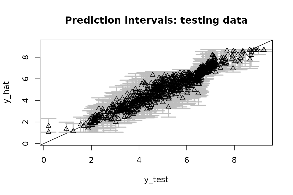
#> [1] 0.929

The out-of-sample predictive distributions are well-calibrated.

Finally, we summarize the posterior inference for the transformation $g$ and the regression coefficients $\theta$ and compare to the ground truth values. First, we plot the posterior draws of $g$ (gray), the posterior mean of $g$ (black), and the true transformation (triangles):

The posterior distribution of $g$ accurately matches the true transformation.

Next, we compute point and interval summaries for $\theta$ and compare them to the ground truth:


# Summarize the parameters (regression coefficients):

# Posterior means:
coef(fit)
#>  [1]  0.07520723  0.47740611  0.44575728  0.48713751  0.34049175  0.39362801
#>  [7]  0.08074457  0.12889488 -0.04967264 -0.08190572  0.08144391

# Check: correlation with true coefficients
cor(dat$beta_true[-1],
    coef(fit)[-1]) # excluding the intercept
#> [1] 0.9431343

# 95% credible intervals:
theta_ci = t(apply(fit$post_theta, 2, quantile, c(.025, 0.975)))

# Check: agreement on nonzero coefficients?
which(theta_ci[,1] >= 0 | theta_ci[,2] <=0) # 95% CI excludes zero
#> [1] 2 3 4 5 6
which(dat$beta_true != 0) # truly nonzero
#> [1] 2 3 4 5 6

The point estimates of $\theta$ closely track the ground truth, and inference based on the 95% credible intervals correctly selects the truly nonzero regression coefficients.

Remark: The location-scale of the data-generating process and the model may not match exactly. Thus, we use correlations to compare the regression coefficients $\theta$ (while omitting the intercept) and apply location-scale shifts of the transformations $g$ to ensure comparability. This is only a byproduct of the simulated data setting and does not matter for real data analysis (or for variable selection).

Note: Try repeating this exercise with blm_bc() in place of sblm(). The Box-Cox transformation cannot recover the transformation $g$ or the coefficients $\theta$ accurately, the model diagnostics are alarming, and the predictions deteriorate substantially.

Semiparametric Bayesian quantile regression with `sbqr`

We now consider Bayesian quantile regression, which specifies a linear model with ALD errors. First, we simulate data from a heteroskedastic linear model. Heteroskedasticity often produces conclusions that differ from traditional mean regression. Here, we do not include a transformation, so the data-generating process does not implicitly favor our approach over traditional Bayesian quantile regression (i.e., with $g(t) = t$ the identity).

# Simulate data from a heteroskedastic linear model (no transformation):
dat = simulate_tlm(n = 200,  # number of observations
                   p = 10,   # number of covariates 
                   g_type = 'box-cox', lambda = 1, # no transformation
                   heterosked = TRUE # heteroskedastic errors
                   )
# Training data:
y = dat$y; X = dat$X 

# Testing data:
y_test = dat$y_test; X_test = dat$X_test

Next, we load in two packages that we’ll need:

library(quantreg) # traditional QR for initialization
library(statmod) # for rinvgauss sampling

Now, we fit two Bayesian quantile regression models: the traditional version without a transformation (bqr()) and the proposed alternative (sbqr()). We target the $\tau = 0.05$ quantile.


# Quantile to target:
tau = 0.05

# (Traditional) Bayesian quantile regression:
fit_bqr = bqr(y = y, 
           X = X, 
           tau = tau, 
           X_test = X_test,
           verbose = FALSE  # omit printout
)

# Semiparametric Bayesian quantile regression:
fit = sbqr(y = y, 
           X = X, 
           tau = tau, 
           X_test = X_test,
           verbose = FALSE # omit printout
)
      
names(fit) # what is returned
#>  [1] "coefficients"  "fitted.values" "post_theta"    "post_ypred"   
#>  [5] "post_qtau"     "post_g"        "model"         "y"            
#>  [9] "X"             "X_test"        "psi"           "approx_g"     
#> [13] "tau"

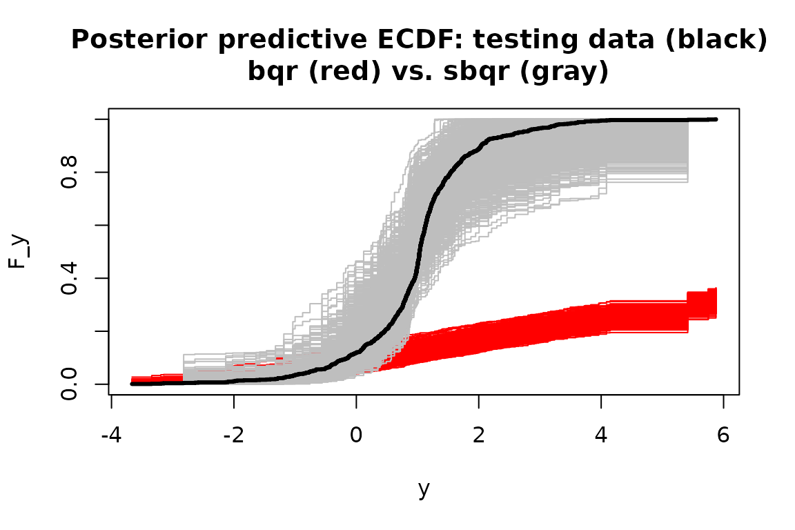
For both model fits, we evaluate the same posterior predictive diagnostics as before. Specifically, we compute the empirical CDF on both y_test (black) and on each simulated testing predictive dataset from post_ypred for sbqr (gray) and bqr (red):

Without the transformation, the Bayesian quantile regression model is not a good model for the data. The learned transformation completely resolves this model inadequacy—even though there was no transformation present in the data-generating process.

Finally, we can asses the quantile estimates on the testing data. First, consider bqr:

# Quantile point estimates:
q_hat_bqr = fitted(fit_bqr) 

# Empirical quantiles on testing data:
(emp_quant_bqr = mean(q_hat_bqr >= y_test))
#> [1] 0.026

# Evaluate posterior predictive means and intervals on the testing data:
(emp_cov_bqr = plot_pptest(fit_bqr$post_ypred, 
                           y_test, 
                           alpha_level = 0.10))

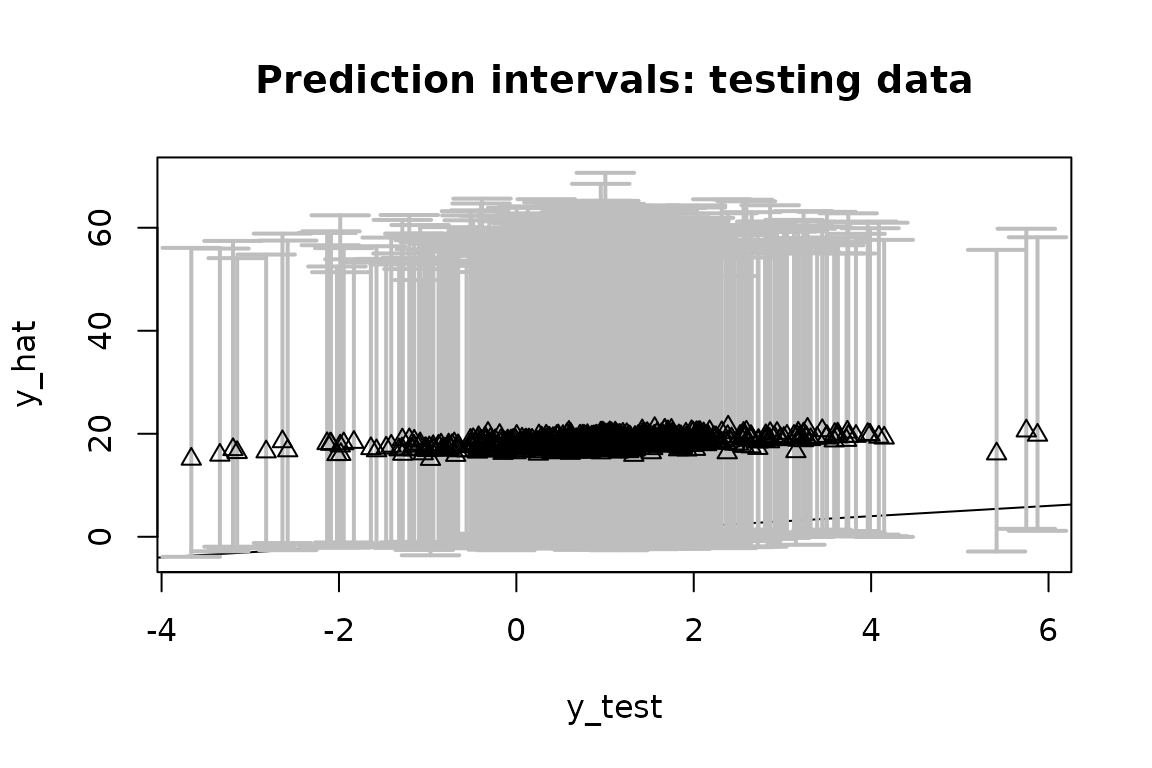
#> [1] 0.98

Recall that these are quantile regression models at $\tau$ , so we expect them to be asymmetric about y_test.

The out-of-sample empirical quantile is 0.026 (the target is $\tau = 0.05$ ) and the 90% prediction interval coverage is 0.98.

Repeat this evaluation for sbqr:

# Quantile point estimates:
q_hat = fitted(fit) 

# Empirical quantiles on testing data:
(emp_quant_sbqr = mean(q_hat >= y_test))
#> [1] 0.034

# Evaluate posterior predictive means and intervals on the testing data:
(emp_cov_sbqr = plot_pptest(fit$post_ypred, 
                            y_test, 
                            alpha_level = 0.10))

#> [1] 0.968

Now the out-of-sample empirical quantile is 0.034 and the 90% prediction interval coverage is 0.968. sbqr is better calibrated to $\tau$ , while both methods are slightly overconservative in the prediction interval coverage. However, sbqr produce significantly smaller prediction intervals while maintaining this conservative coverage, and thus provides more powerful and precise inference.

Remark: point and interval estimates for the quantile regression coefficients $\theta$ may be computed exactly as in the sblm() example.

Note: try this again for other quantiles, such as $\tau \in\{0.25, 0.5\}$ . As $\tau$ approaches 0.5 (i.e., median regression), the problem becomes easier and the models are better calibrated.

Semiparametric Bayesian Gaussian processes with `sbgp`

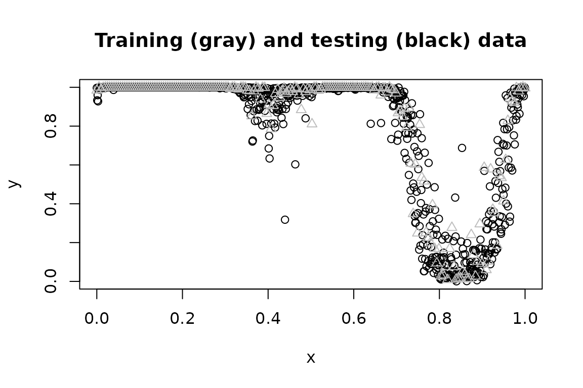
Consider a challenging scenario with (i) a nonlinear regression function of $x \in \mathbb{R}$ and (ii) Beta marginals, so the support is $\mathcal{Y} = [0,1]$ . Simulate data accordingly:

# Training data:
n = 200 # sample size
x = seq(0, 1, length = n) # observation points

# Testing data:
n_test = 1000 
x_test = seq(0, 1, length = n_test) 

# True inverse transformation:
g_inv_true = function(z) 
  qbeta(pnorm(z), 
        shape1 = 0.5, 
        shape2 = 0.1) # approx Beta(0.5, 0.1) marginals

# Training observations:
y = g_inv_true(
  sin(2*pi*x) + sin(4*pi*x) + .25*rnorm(n)
             ) 

# Testing observations:
y_test = g_inv_true(
  sin(2*pi*x_test) + sin(4*pi*x_test) + .25*rnorm(n)
             ) 

plot(x_test, y_test, 
     xlab = 'x', ylab = 'y',
     main = "Training (gray) and testing (black) data")
lines(x, y, type='p', col='gray', pch = 2)

To highlight the challenges here, we first consider a Box-Cox-transformed GP. For this as well as the proposed model, we require a package:

library(GpGp) # fast GP computing
library(fields) # accompanies GpGp

Now we fit the Box-Cox GP and evaluate the out-of-sample predictive performance:

# Fit the Box-Cox Gaussian process model:
fit_bc = bgp_bc(y = y, 
           locs = x,
           locs_test = x_test)
#> [1] "Initial GP fit..."
#> [1] "Updated GP fit..."

# Fitted values on the testing data:
y_hat_bc = fitted(fit_bc)

# 90% prediction intervals on the testing data:
pi_y_bc = t(apply(fit_bc$post_ypred, 2, quantile, c(0.05, .95))) 

# Average PI width:
(width_bc = mean(pi_y_bc[,2] - pi_y_bc[,1]))
#> [1] 0.2668766

# Empirical PI coverage:
(emp_cov_bc = mean((pi_y_bc[,1] <= y_test)*(pi_y_bc[,2] >= y_test)))
#> [1] 0.894

# Plot these together with the actual testing points:
plot(x_test, y_test, type='n', 
     ylim = range(pi_y_bc, y_test), xlab = 'x', ylab = 'y', 
     main = paste('Fitted values and prediction intervals: \n Box-Cox Gaussian process'))

# Add the intervals:
polygon(c(x_test, rev(x_test)),
        c(pi_y_bc[,2], rev(pi_y_bc[,1])),
        col='gray', border=NA)
lines(x_test, y_test, type='p') # actual values
lines(x_test, y_hat_bc, lwd = 3) # fitted values

The Box-Cox transformation adds some flexibility to the GP, but is insufficient for these data. The prediction intervals are unnecessarily wide and do not respect the support $\mathcal{Y} = [0,1]$ , while the estimated mean function does not fully capture the trend in the data.

Now fit the semiparametric Bayesian GP model:


# library(GpGp) # loaded above

# Fit the semiparametric Gaussian process model:
fit = sbgp(y = y, 
           locs = x,
           locs_test = x_test)
#> [1] "Initial GP fit..."
#> [1] "Updated GP fit..."
#> [1] "Sampling..."
#> [1] "Done!"

names(fit) # what is returned
#>  [1] "coefficients"  "fitted.values" "fit_gp"        "post_ypred"   
#>  [5] "post_g"        "model"         "y"             "X"            
#>  [9] "approx_g"      "sigma_epsilon"

coef(fit) # estimated regression coefficients (here, just an intercept)
#> [1] 0.02256626

Evaluate the out-of-sample predictive performance on the testing data:

# Fitted values on the testing data:
y_hat = fitted(fit)

# 90% prediction intervals on the testing data:
pi_y = t(apply(fit$post_ypred, 2, quantile, c(0.05, .95))) 

# Average PI width:
(width = mean(pi_y[,2] - pi_y[,1]))
#> [1] 0.2150783

# Empirical PI coverage:
(emp_cov = mean((pi_y[,1] <= y_test)*(pi_y[,2] >= y_test)))
#> [1] 0.955

# Plot these together with the actual testing points:
plot(x_test, y_test, type='n', 
     ylim = range(pi_y, y_test), xlab = 'x', ylab = 'y', 
     main = paste('Fitted values and prediction intervals: \n semiparametric Gaussian process'))

# Add the intervals:
polygon(c(x_test, rev(x_test)),
        c(pi_y[,2], rev(pi_y[,1])),
        col='gray', border=NA)
lines(x_test, y_test, type='p') # actual values
lines(x_test, y_hat, lwd = 3) # fitted values

Unlike the Box-Cox version, sbgp respects the support of the data $\mathcal{Y} = [0,1]$ , captures the trend, and provides narrower intervals (average widths are 0.215 compared to 0.267) with better coverage (0.955 for sbgp and 0.894 for Box-Cox).

Despite the significant complexities in the data, sbgp performs quite well out-of-the-box:

the nonlinearity is modeled adequately;
the support of the data is enforced automatically;
the out-of-sample prediction intervals are sharp and calibrated; and
the computations are fast.

Note: sbgp also applies for $x \in \mathbb{R}^p$ with $p >1$ , such as spatial or spatio-temporal data. Such cases may require more careful consideration of the mean and covariance functions: the default mean function is a linear regression with the intercept only, while the default covariance function is an isotropic Matern function. However, many other options are available (inherited from the GpGp package).

References

Kowal, D. and Wu, B. (2024). Monte Carlo inference for semiparametric Bayesian regression. JASA. https://doi.org/10.1080/01621459.2024.2395586

Background: semiparametric regression via data transformations

Using SeBR

Semiparametric Bayesian linear models with sblm

Semiparametric Bayesian quantile regression with sbqr

Semiparametric Bayesian Gaussian processes with sbgp

References

Using `SeBR`

Semiparametric Bayesian linear models with `sblm`

Semiparametric Bayesian quantile regression with `sbqr`

Semiparametric Bayesian Gaussian processes with `sbgp`