MCMC sampling for Bayesian spline regression with a (known or unknown) Box-Cox transformation.
Usage
bsm_bc(
  y,
  x = NULL,
  x_test = x,
  psi = NULL,
  lambda = NULL,
  sample_lambda = TRUE,
  nsave = 1000,
  nburn = 1000,
  nskip = 0,
  verbose = TRUE
)
Arguments
- y
n x 1vector of observed counts- x
n x 1vector of observation points; if NULL, assume equally-spaced on [0,1]- x_test
n_test x 1vector of testing points; if NULL, assume equal tox- psi
prior variance (inverse smoothing parameter); if NULL, sample this parameter
- lambda
Box-Cox transformation; if NULL, estimate this parameter
- sample_lambda
logical; if TRUE, sample lambda, otherwise use the fixed value of lambda above or the MLE (if lambda unspecified)
- nsave
number of MCMC iterations to save
- nburn
number of MCMC iterations to discard
- nskip
number of MCMC iterations to skip between saving iterations, i.e., save every (nskip + 1)th draw
- verbose
logical; if TRUE, print time remaining
Value
a list with the following elements:
coefficientsthe posterior mean of the regression coefficientsfitted.valuesthe posterior predictive mean at the test pointsx_testpost_theta:nsave x psamples from the posterior distribution of the regression coefficientspost_ypred:nsave x n_testsamples from the posterior predictive distribution atx_testpost_g:nsaveposterior samples of the transformation evaluated at the uniqueyvaluespost_lambdansaveposterior samples of lambdamodel: the model fit (here,sbsm_bc)
as well as the arguments passed in.
Details
This function provides fully Bayesian inference for a
transformed spline model via MCMC sampling. The transformation is
parametric from the Box-Cox family, which has one parameter lambda.
That parameter may be fixed in advanced or learned from the data.
Note
Box-Cox transformations may be useful in some cases, but
in general we recommend the nonparametric transformation (with
Monte Carlo, not MCMC sampling) in sbsm.
Examples
# Simulate some data:
n = 100 # sample size
x = sort(runif(n)) # observation points
# Transform a noisy, periodic function:
y = g_inv_bc(
sin(2*pi*x) + sin(4*pi*x) + rnorm(n, sd = .5),
lambda = .5) # Signed square-root transformation
# Fit the Bayesian spline model with a Box-Cox transformation:
fit = bsm_bc(y = y, x = x)
#> [1] "1 sec remaining"
#> [1] "1 sec remaining"
#> [1] "Total time: 0 seconds"
names(fit) # what is returned
#> [1] "coefficients" "fitted.values" "post_theta" "post_ypred"
#> [5] "post_g" "post_lambda" "model" "y"
#> [9] "X" "psi"
round(quantile(fit$post_lambda), 3) # summary of unknown Box-Cox parameter
#> 0% 25% 50% 75% 100%
#> 0.517 0.652 0.697 0.739 0.882
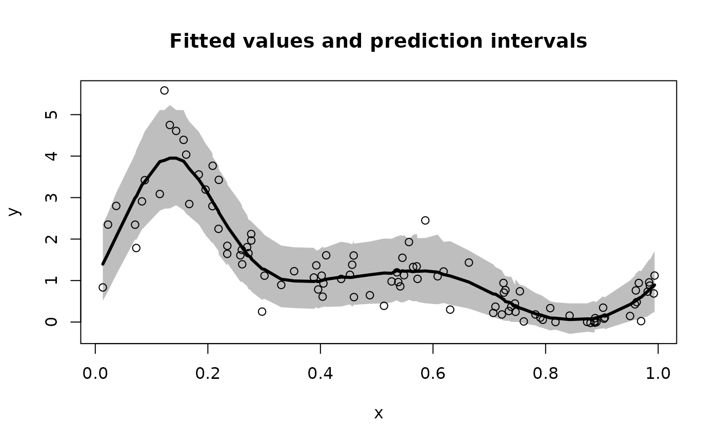
# Plot the model predictions (point and interval estimates):
pi_y = t(apply(fit$post_ypred, 2, quantile, c(0.05, .95))) # 90% PI
plot(x, y, type='n', ylim = range(pi_y,y),
xlab = 'x', ylab = 'y', main = paste('Fitted values and prediction intervals'))
polygon(c(x, rev(x)),c(pi_y[,2], rev(pi_y[,1])),col='gray', border=NA)
lines(x, y, type='p')
lines(x, fitted(fit), lwd = 3)