Monte Carlo sampling for Bayesian Gaussian process regression with an unknown (nonparametric) transformation.
Usage
sbgp(
  y,
  locs,
  X = NULL,
  covfun_name = "matern_isotropic",
  locs_test = locs,
  X_test = NULL,
  nn = 30,
  fixedX = (length(y) >= 500),
  approx_g = FALSE,
  samp_losc = TRUE,
  nsave = 1000,
  ngrid = 100
)
Arguments
- y
n x 1response vector- locs
n x dmatrix of locations- X
n x pdesign matrix; if unspecified, use intercept only- covfun_name
string name of a covariance function; see ?GpGp
- locs_test
n_test x dmatrix of locations at which predictions are needed; default islocs- X_test
n_test x pdesign matrix for test data; default isX- nn
number of nearest neighbors to use; default is 30 (larger values improve the GP approximation but increase computing cost)
- fixedX
logical; if TRUE, treat the design as fixed (non-random) when sampling the transformation; otherwise treat covariates as random with an unknown distribution
- approx_g
logical; if TRUE, apply large-sample approximation for the transformation
- samp_losc
logical; if TRUE, apply location-scale sampling adjustment
- nsave
number of Monte Carlo simulations
- ngrid
number of grid points for inverse approximations
Value
a list with the following elements:
coefficientsthe estimated regression coefficientsfitted.valuesthe posterior predictive mean at the test pointslocs_testfit_gpthe fittedGpGp_fitobject, which includes covariance parameter estimates and other model informationpost_ypred:nsave x ntestsamples from the posterior predictive distribution atlocs_testpost_g:nsaveposterior samples of the transformation evaluated at the uniqueyvaluesmodel: the model fit (here,sbgp)
as well as the arguments passed in.
Details
This function provides Bayesian inference for a
transformed Gaussian process model using Monte Carlo (not MCMC) sampling.
The transformation is modeled as unknown (unless approx_g = TRUE,
which then uses a point approximation) and learned jointly
with the regression function. This model applies for real-valued data, positive data, and
compactly-supported data (the support is automatically deduced from the observed y values).
The results are typically unchanged whether laplace_approx is TRUE/FALSE;
setting it to TRUE may reduce sensitivity to the prior, while setting it to FALSE
may speed up computations for very large datasets. For computational efficiency,
the Gaussian process parameters and curve estimates are fixed at point estimates.
However, the accompanying uncertainties are often negligible compared to the observation errors, and the
transformation serves as an additional layer of robustness. By default, fixedX is
set to FALSE for smaller datasets (n < 500) and TRUE for larger datasets (n >= 500).
Examples
# \donttest{
# Simulate some data:
n = 200 # sample size
x = seq(0, 1, length = n) # observation points
# Transform a noisy, periodic function:
y = g_inv_bc(
sin(2*pi*x) + sin(4*pi*x) + rnorm(n),
lambda = .5) # Signed square-root transformation
# Package we use for fast computing w/ Gaussian processes:
library(GpGp)
# Fit the semiparametric Bayesian Gaussian process:
fit = sbgp(y = y, locs = x)
#> [1] "Initial GP fit..."
#> [1] "Updated GP fit..."
#> [1] "Sampling..."
#> [1] "Done!"
names(fit) # what is returned
#> [1] "coefficients" "fitted.values" "fit_gp" "post_ypred"
#> [5] "post_g" "model" "y" "X"
#> [9] "X_test" "nn" "fixedX" "approx_g"
#> [13] "samp_losc"
coef(fit) # estimated regression coefficients (here, just an intercept)
#> [1] 0.005523801
class(fit$fit_gp) # the GpGp object is also returned
#> [1] "GpGp_fit"
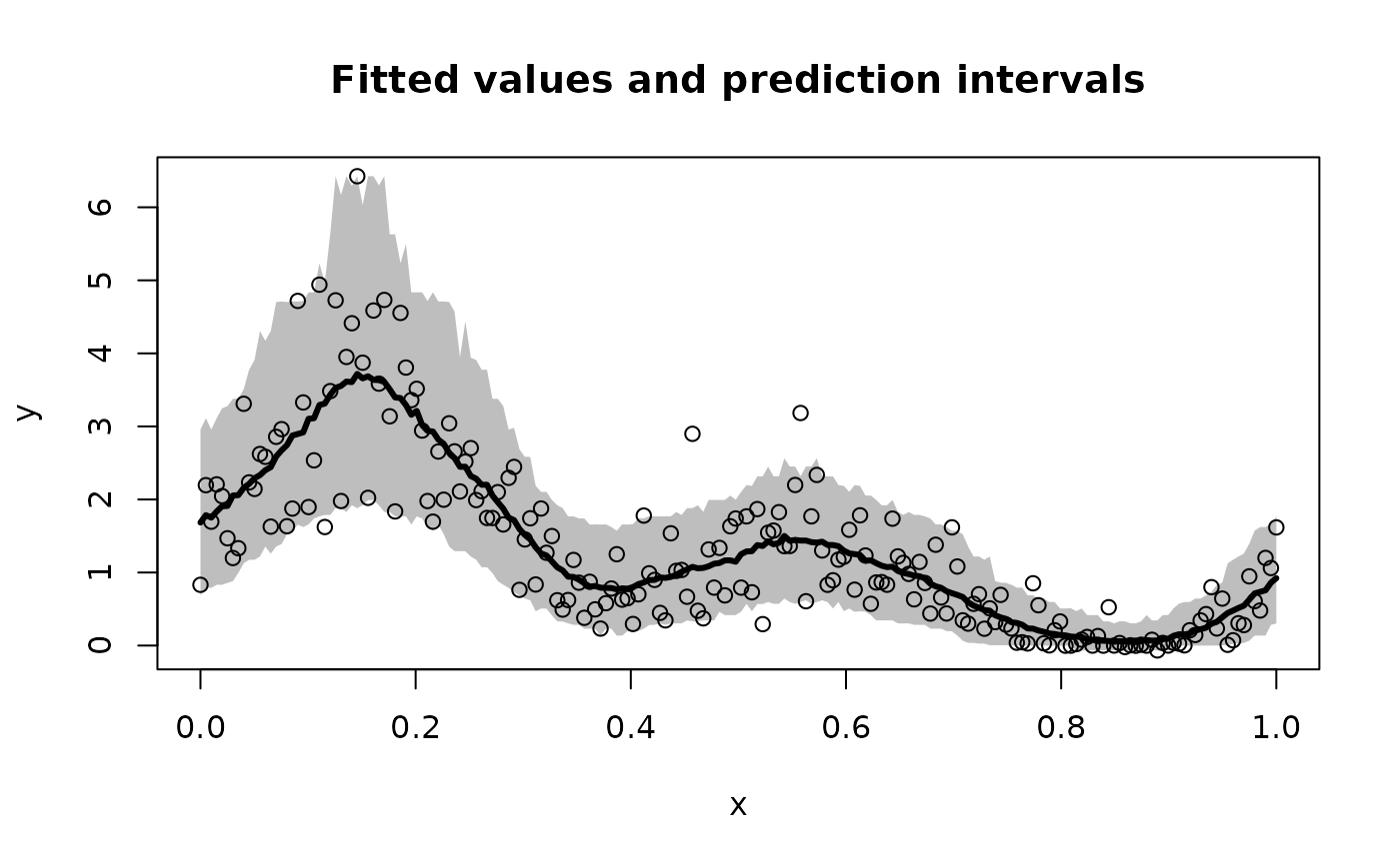
# Plot the model predictions (point and interval estimates):
pi_y = t(apply(fit$post_ypred, 2, quantile, c(0.05, .95))) # 90% PI
plot(x, y, type='n', ylim = range(pi_y,y),
xlab = 'x', ylab = 'y', main = paste('Fitted values and prediction intervals'))
polygon(c(x, rev(x)),c(pi_y[,2], rev(pi_y[,1])),col='gray', border=NA)
lines(x, y, type='p') # observed points
lines(x, fitted(fit), lwd = 3) # fitted curve
 # }
# }