MCMC sampling for Bayesian Gaussian process regression with a (known or unknown) Box-Cox transformation.
Usage
bgp_bc(
  y,
  locs,
  X = NULL,
  covfun_name = "matern_isotropic",
  locs_test = locs,
  X_test = NULL,
  nn = 30,
  emp_bayes = TRUE,
  lambda = NULL,
  sample_lambda = TRUE,
  nsave = 1000,
  nburn = 1000,
  nskip = 0
)
Arguments
- y
n x 1response vector- locs
n x dmatrix of locations- X
n x pdesign matrix; if unspecified, use intercept only- covfun_name
string name of a covariance function; see ?GpGp
- locs_test
n_test x dmatrix of locations at which predictions are needed; default islocs- X_test
n_test x pdesign matrix for test data; default isX- nn
number of nearest neighbors to use; default is 30 (larger values improve the approximation but increase computing cost)
- emp_bayes
logical; if TRUE, use a (faster!) empirical Bayes approach for estimating the mean function
- lambda
Box-Cox transformation; if NULL, estimate this parameter
- sample_lambda
logical; if TRUE, sample lambda, otherwise use the fixed value of lambda above or the MLE (if lambda unspecified)
- nsave
number of MCMC iterations to save
- nburn
number of MCMC iterations to discard
- nskip
number of MCMC iterations to skip between saving iterations, i.e., save every (nskip + 1)th draw
Value
a list with the following elements:
coefficientsthe posterior mean of the regression coefficientsfitted.valuesthe posterior predictive mean at the test pointslocs_testfit_gpthe fittedGpGp_fitobject, which includes covariance parameter estimates and other model informationpost_ypred:nsave x n_testsamples from the posterior predictive distribution atlocs_testpost_g:nsaveposterior samples of the transformation evaluated at the uniqueyvaluespost_lambdansaveposterior samples of lambdamodel: the model fit (here,bgp_bc)
as well as the arguments passed in.
Details
This function provides Bayesian inference for
transformed Gaussian processes. The transformation is
parametric from the Box-Cox family, which has one parameter lambda.
That parameter may be fixed in advanced or learned from the data.
For computational efficiency, the Gaussian process parameters are
fixed at point estimates, and the latent Gaussian process is only sampled
when emp_bayes = FALSE.
Note
Box-Cox transformations may be useful in some cases, but
in general we recommend the nonparametric transformation (with
Monte Carlo, not MCMC sampling) in sbgp.
Examples
# \donttest{
# Simulate some data:
n = 200 # sample size
x = seq(0, 1, length = n) # observation points

# Transform a noisy, periodic function:
y = g_inv_bc(
  sin(2*pi*x) + sin(4*pi*x) + rnorm(n, sd = .5),
             lambda = .5) # Signed square-root transformation

# Package we use for fast computing w/ Gaussian processes:
library(GpGp)

# Fit a Bayesian Gaussian process with Box-Cox transformation:
fit = bgp_bc(y = y, locs = x)
#> [1] "Initial GP fit..."
#> [1] "Updated GP fit..."
names(fit) # what is returned
#> [1] "coefficients"  "fitted.values" "fit_gp"        "post_ypred"
#> [5] "post_g"        "post_lambda"   "model"         "y"
#> [9] "X"
coef(fit) # estimated regression coefficients (here, just an intercept)
#> [1] 0.2221119
class(fit$fit_gp) # the GpGp object is also returned
#> [1] "GpGp_fit"
round(quantile(fit$post_lambda), 3) # summary of unknown Box-Cox parameter
#>    0%   25%   50%   75%  100%
#> 0.681 0.779 0.805 0.832 0.922

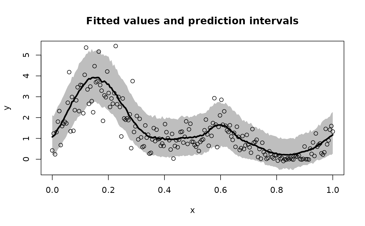
# Plot the model predictions (point and interval estimates):
pi_y = t(apply(fit$post_ypred, 2, quantile, c(0.05, .95))) # 90% PI
plot(x, y, type='n', ylim = range(pi_y,y),
     xlab = 'x', ylab = 'y', main = paste('Fitted values and prediction intervals'))
polygon(c(x, rev(x)),c(pi_y[,2], rev(pi_y[,1])),col='gray', border=NA)
lines(x, y, type='p')
lines(x, fitted(fit), lwd = 3)

# }
# }