Plot point and interval predictions on testing data

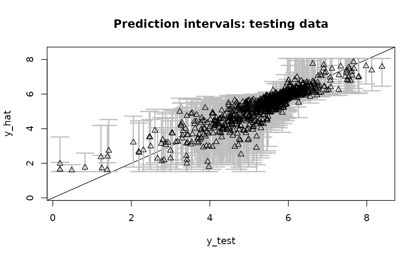
Given posterior predictive samples at X_test, plot the point and interval estimates and compare to the actual testing data y_test.

Usage

plot_pptest(post_ypred, y_test, alpha_level = 0.1)

Arguments

post_ypred

nsave x n_test samples from the posterior predictive distribution at test points X_test

y_test

n_test testing points

alpha_level

alpha-level for prediction intervals

Value

plot of the testing data, point and interval predictions, and a summary of the empirical coverage

Examples

# \donttest{
# Simulate some data:
dat = simulate_tlm(n = 100, p = 5, g_type = 'step')

# Fit a semiparametric Bayesian linear model:
fit = sblm(y = dat$y, X = dat$X, X_test = dat$X_test)
#> [1] "4 seconds remaining"
#> [1] "3 seconds remaining"
#> [1] "2 seconds remaining"
#> [1] "Total time:  5 seconds"

# Evaluate posterior predictive means and intervals on the testing data:
plot_pptest(fit$post_ypred, dat$y_test,
            alpha_level = 0.10) # coverage should be about 90%

#> [1] 0.888
# }