Monte Carlo sampling for Bayesian linear regression with an unknown (nonparametric) transformation. A g-prior is assumed for the regression coefficients.
Arguments
- y
n x 1response vector- X
n x pmatrix of predictors (no intercept)- X_test
n_test x pmatrix of predictors for test data; default is the observed covariatesX- psi
prior variance (g-prior)
- laplace_approx
logical; if TRUE, use a normal approximation to the posterior in the definition of the transformation; otherwise the prior is used
- fixedX
logical; if TRUE, treat the design as fixed (non-random) when sampling the transformation; otherwise treat covariates as random with an unknown distribution
- approx_g
logical; if TRUE, apply large-sample approximation for the transformation
- nsave
number of Monte Carlo simulations
- ngrid
number of grid points for inverse approximations
- verbose
logical; if TRUE, print time remaining
Value
a list with the following elements:
coefficientsthe posterior mean of the regression coefficientsfitted.valuesthe posterior predictive mean at the test pointsX_testpost_theta:nsave x psamples from the posterior distribution of the regression coefficientspost_ypred:nsave x n_testsamples from the posterior predictive distribution at test pointsX_testpost_g:nsaveposterior samples of the transformation evaluated at the uniqueyvaluesmodel: the model fit (here,sblm)
as well as the arguments passed in.
Details
This function provides fully Bayesian inference for a
transformed linear model using Monte Carlo (not MCMC) sampling.
The transformation is modeled as unknown and learned jointly
with the regression coefficients (unless approx_g = TRUE, which then uses
a point approximation). This model applies for real-valued data, positive data, and
compactly-supported data (the support is automatically deduced from the observed y values).
The results are typically unchanged whether laplace_approx is TRUE/FALSE;
setting it to TRUE may reduce sensitivity to the prior, while setting it to FALSE
may speed up computations for very large datasets. By default, fixedX is
set to FALSE for smaller datasets (n < 500) and TRUE for larger datasets (n >= 500).
Note
The location (intercept) and scale (sigma_epsilon) are
not identified, so any intercepts in X and X_test will
be removed. The model-fitting *does* include an internal location-scale
adjustment, but the function only outputs inferential summaries for the
identifiable parameters.
Examples
# \donttest{
# Simulate some data:
dat = simulate_tlm(n = 100, p = 5, g_type = 'step')
y = dat$y; X = dat$X # training data
y_test = dat$y_test; X_test = dat$X_test # testing data
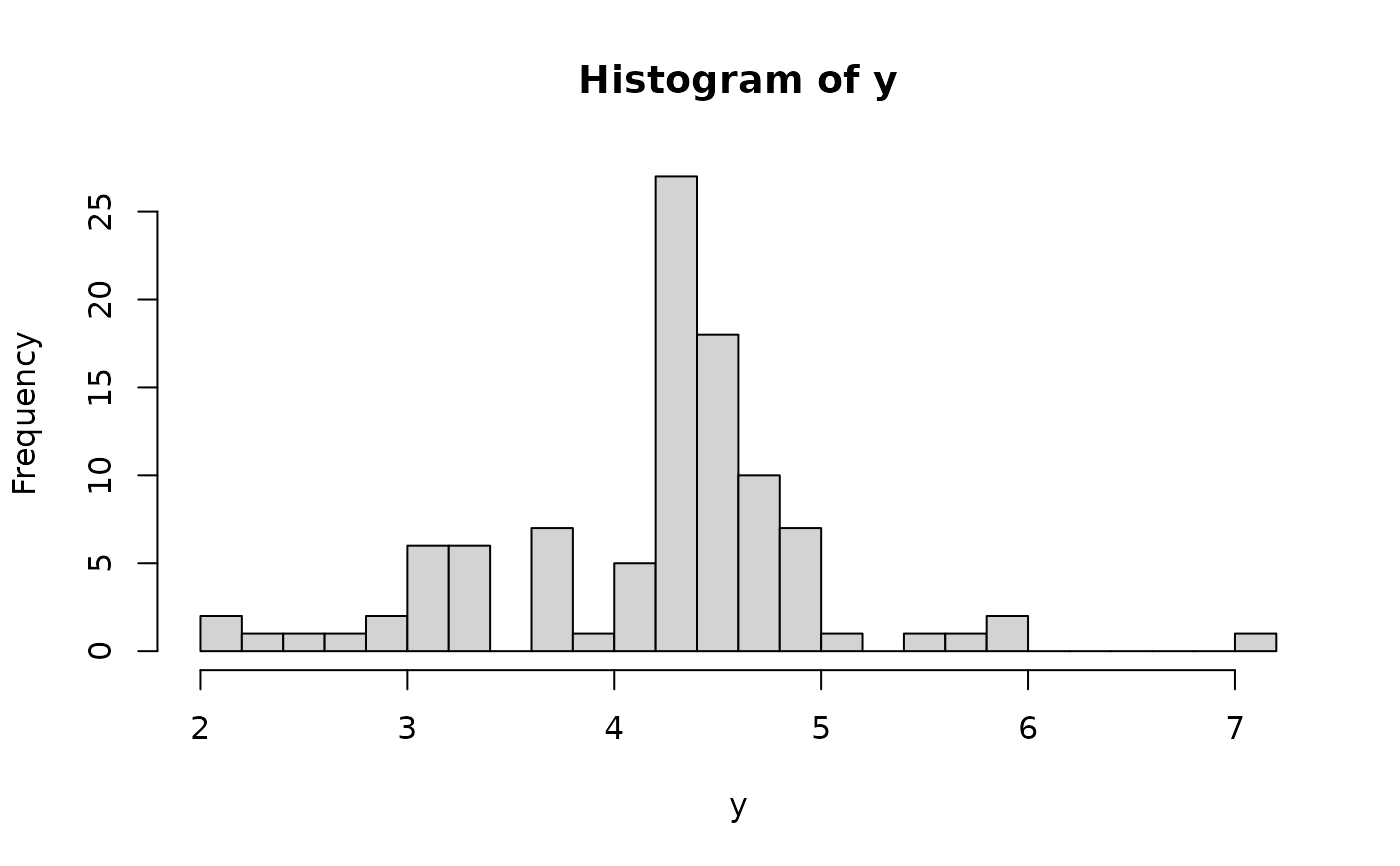
hist(y, breaks = 25) # marginal distribution
 # Fit the semiparametric Bayesian linear model:
fit = sblm(y = y, X = X, X_test = X_test)
#> [1] "3 sec remaining"
#> [1] "2 sec remaining"
#> [1] "Total time: 3 seconds"
names(fit) # what is returned
#> [1] "coefficients" "fitted.values" "post_theta" "post_ypred"
#> [5] "post_g" "model" "y" "X"
#> [9] "X_test" "psi" "laplace_approx" "fixedX"
#> [13] "approx_g"
# Note: this is Monte Carlo sampling...no need for MCMC diagnostics!
# Evaluate posterior predictive means and intervals on the testing data:
plot_pptest(fit$post_ypred, y_test,
alpha_level = 0.10) # coverage should be about 90%
# Fit the semiparametric Bayesian linear model:
fit = sblm(y = y, X = X, X_test = X_test)
#> [1] "3 sec remaining"
#> [1] "2 sec remaining"
#> [1] "Total time: 3 seconds"
names(fit) # what is returned
#> [1] "coefficients" "fitted.values" "post_theta" "post_ypred"
#> [5] "post_g" "model" "y" "X"
#> [9] "X_test" "psi" "laplace_approx" "fixedX"
#> [13] "approx_g"
# Note: this is Monte Carlo sampling...no need for MCMC diagnostics!
# Evaluate posterior predictive means and intervals on the testing data:
plot_pptest(fit$post_ypred, y_test,
alpha_level = 0.10) # coverage should be about 90%
 #> [1] 0.876
# Check: correlation with true coefficients
cor(dat$beta_true, coef(fit))
#> [1] 0.9448987
# Summarize the transformation:
y0 = sort(unique(y)) # posterior draws of g are evaluated at the unique y observations
plot(y0, fit$post_g[1,], type='n', ylim = range(fit$post_g),
xlab = 'y', ylab = 'g(y)', main = "Posterior draws of the transformation")
temp = sapply(1:nrow(fit$post_g), function(s)
lines(y0, fit$post_g[s,], col='gray')) # posterior draws
lines(y0, colMeans(fit$post_g), lwd = 3) # posterior mean
lines(y, dat$g_true, type='p', pch=2) # true transformation
legend('bottomright', c('Truth'), pch = 2) # annotate the true transformation
#> [1] 0.876
# Check: correlation with true coefficients
cor(dat$beta_true, coef(fit))
#> [1] 0.9448987
# Summarize the transformation:
y0 = sort(unique(y)) # posterior draws of g are evaluated at the unique y observations
plot(y0, fit$post_g[1,], type='n', ylim = range(fit$post_g),
xlab = 'y', ylab = 'g(y)', main = "Posterior draws of the transformation")
temp = sapply(1:nrow(fit$post_g), function(s)
lines(y0, fit$post_g[s,], col='gray')) # posterior draws
lines(y0, colMeans(fit$post_g), lwd = 3) # posterior mean
lines(y, dat$g_true, type='p', pch=2) # true transformation
legend('bottomright', c('Truth'), pch = 2) # annotate the true transformation
 # Posterior predictive checks on testing data: empirical CDF
y0 = sort(unique(y_test))
plot(y0, y0, type='n', ylim = c(0,1),
xlab='y', ylab='F_y', main = 'Posterior predictive ECDF')
temp = sapply(1:nrow(fit$post_ypred), function(s)
lines(y0, ecdf(fit$post_ypred[s,])(y0), # ECDF of posterior predictive draws
col='gray', type ='s'))
lines(y0, ecdf(y_test)(y0), # ECDF of testing data
col='black', type = 's', lwd = 3)
# Posterior predictive checks on testing data: empirical CDF
y0 = sort(unique(y_test))
plot(y0, y0, type='n', ylim = c(0,1),
xlab='y', ylab='F_y', main = 'Posterior predictive ECDF')
temp = sapply(1:nrow(fit$post_ypred), function(s)
lines(y0, ecdf(fit$post_ypred[s,])(y0), # ECDF of posterior predictive draws
col='gray', type ='s'))
lines(y0, ecdf(y_test)(y0), # ECDF of testing data
col='black', type = 's', lwd = 3)
 # }
# }