Given Monte Carlo draws from the surrogate posterior, apply sampling importance reweighting (SIR) to correct for the true model likelihood.
Arguments
- fit
a fitted model object that includes
coefficientsthe posterior mean of the regression coefficientspost_theta:nsave x psamples from the posterior distribution of the regression coefficientspost_ypred:nsave x n_testsamples from the posterior predictive distribution at test pointsX_testpost_g:nsaveposterior samples of the transformation evaluated at the uniqueyvaluesmodel: the model fit (sblmorsbsm)
- sir_frac
fraction of draws to sample for SIR
- nsims_prior
number of draws from the prior
- marg_x
logical; if TRUE, compute the weights marginal over the covariates
- verbose
logical; if TRUE, print time remaining
Details
The Monte Carlo sampling for sblm and
sbsm uses a surrogate likelihood for posterior inference,
which enables much faster and easier computing. SIR provides a correction for
the actual (specified) likelihood. However, this correction
step typically does not produce any noticeable
discrepancies, even for small sample sizes.
Note
SIR sampling is done *without* replacement, so sir_frac
is typically between 0.1 and 0.5. The nsims_priors draws
are used to approximate a prior expectation, but larger values
can significantly slow down this function. The importance weights
can be computed conditionally (marg_x = FALSE) or unconditionally
(marg_x = TRUE) on the covariates, corresponding to whether
or not the covariates are marginalized out in the likelihood. The
conditional version is much faster.
Examples
# \donttest{
# Simulate some data:
dat = simulate_tlm(n = 50, p = 5, g_type = 'step')
y = dat$y; X = dat$X # training data
y_test = dat$y_test; X_test = dat$X_test # testing data

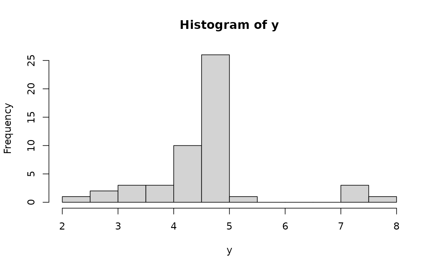
hist(y, breaks = 10) # marginal distribution


# Fit the semiparametric Bayesian linear model:
fit = sblm(y = y, X = X, X_test = X_test)
#> [1] "2 sec remaining"
#> [1] "1 sec remaining"
#> [1] "Total time: 3 seconds"
names(fit) # what is returned
#>  [1] "coefficients"   "fitted.values"  "post_theta"     "post_ypred"
#>  [5] "post_g"         "model"          "y"              "X"
#>  [9] "X_test"         "psi"            "laplace_approx" "fixedX"
#> [13] "approx_g"

# Update with SIR:
fit_sir = sir_adjust(fit)
#> [1] "1 sec remaining"
#> [1] "1 sec remaining"
#> [1] "Total time: 1 seconds"
names(fit_sir) # what is returned
#>  [1] "coefficients"   "fitted.values"  "post_theta"     "post_ypred"
#>  [5] "post_g"         "model"          "y"              "X"
#>  [9] "X_test"         "psi"            "laplace_approx" "fixedX"
#> [13] "approx_g"

# Prediction: unadjusted vs. adjusted?

# Point estimates:
y_hat = fitted(fit)
y_hat_sir = fitted(fit_sir)
cor(y_hat, y_hat_sir) # similar
#> [1] 0.9995179

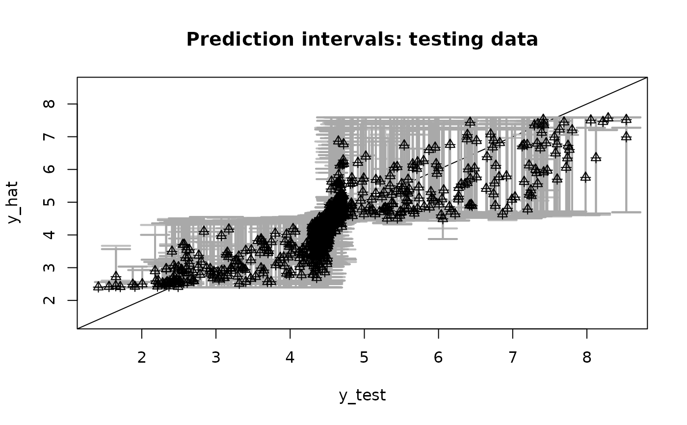
# Interval estimates:
pi_y = t(apply(fit$post_ypred, 2, quantile, c(0.05, .95))) # 90% PI
pi_y_sir = t(apply(fit_sir$post_ypred, 2, quantile, c(0.05, .95))) # 90% PI

# PI overlap (%):
overlaps = 100*sapply(1:length(y_test), function(i){
  # innermost part
  (min(pi_y[i,2], pi_y_sir[i,2]) - max(pi_y[i,1], pi_y_sir[i,1]))/
    # outermost part
    (max(pi_y[i,2], pi_y_sir[i,2]) - min(pi_y[i,1], pi_y_sir[i,1]))
})
summary(overlaps) # mostly close to 100%
#>    Min. 1st Qu.  Median    Mean 3rd Qu.    Max.    NA's
#>   37.63   79.68   90.65   86.59   96.94  100.00       1

# Coverage of PIs on testing data (should be ~ 90%)
mean((pi_y[,1] <= y_test)*(pi_y[,2] >= y_test)) # unadjusted
#> [1] 0.882
mean((pi_y_sir[,1] <= y_test)*(pi_y_sir[,2] >= y_test)) # adjusted
#> [1] 0.832

# Plot together with testing data:
plot(y_test, y_test, type='n', ylim = range(pi_y, pi_y_sir, y_test),
     xlab = 'y_test', ylab = 'y_hat', main = paste('Prediction intervals: testing data'))
abline(0,1) # reference line
suppressWarnings(
  arrows(y_test, pi_y[,1], y_test, pi_y[,2],
         length=0.15, angle=90, code=3, col='gray', lwd=2)
) # plot the PIs (unadjusted)
suppressWarnings(
  arrows(y_test, pi_y_sir[,1], y_test, pi_y_sir[,2],
         length=0.15, angle=90, code=3, col='darkgray', lwd=2)
) # plot the PIs (adjusted)
lines(y_test, y_hat, type='p', pch=2) # plot the means (unadjusted)
lines(y_test, y_hat_sir, type='p', pch=3) # plot the means (adjusted)

# }
# }