Semiparametric Bayesian linear model with stochastic search variable selection
Source:R/source_varsel.R
sblm_ssvs.RdMCMC sampling for semiparametric Bayesian linear regression with
1) an unknown (nonparametric) transformation and 2) a sparsity prior on
the (possibly high-dimensional) regression coefficients. Here, unlike sblm,
Gibbs sampling is used for the variable inclusion indicator variables
gamma, referred to as stochastic search variable selection (SSVS).
All remaining terms–including the transformation g, the regression
coefficients theta, and any predictive draws–are drawn directly from
the joint posterior (predictive) distribution.
Arguments
- y
n x 1response vector- X
n x pmatrix of predictors (no intercept)- X_test
n_test x pmatrix of predictors for test data; default is the observed covariatesX- psi
prior variance (g-prior)
- fixedX
logical; if TRUE, treat the design as fixed (non-random) when sampling the transformation; otherwise treat covariates as random with an unknown distribution
- approx_g
logical; if TRUE, apply large-sample approximation for the transformation
- init_screen
for the initial approximation, number of covariates to pre-screen (necessary when
p > n); if NULL, usen/log(n)- a_pi
shape1 parameter of the (Beta) prior inclusion probability
- b_pi
shape2 parameter of the (Beta) prior inclusion probability
- nsave
number of MCMC simulations to save
- nburn
number of MCMC iterations to discard
- ngrid
number of grid points for inverse approximations
- verbose
logical; if TRUE, print time remaining
Value
a list with the following elements:
coefficientsthe posterior mean of the regression coefficientsfitted.valuesthe posterior predictive mean at the test pointsX_testselected: the variables (columns ofX) selected by the median probability modelpip: (marginal) posterior inclusion probabilities for each variablepost_theta:nsave x psamples from the posterior distribution of the regression coefficientspost_gamma:nsave x psamples from the posterior distribution of the variable inclusion indicatorspost_ypred:nsave x n_testsamples from the posterior predictive distribution at test pointsX_testpost_g:nsaveposterior samples of the transformation evaluated at the uniqueyvaluesmodel: the model fit (here,sblm_ssvs)
as well as the arguments passed in.
Details
This function provides fully Bayesian inference for a
transformed linear model with sparse g-priors on the regression coefficients.
The transformation is modeled as unknown and learned jointly
with the regression coefficients (unless approx_g = TRUE, which then uses
a point approximation). This model applies for real-valued data, positive data, and
compactly-supported data (the support is automatically deduced from the observed y values).
By default, fixedX is set to FALSE for smaller datasets (n < 500)
and TRUE for larger datasets.
The sparsity prior is especially useful for variable selection. Compared
to the horseshoe prior version (sblm_hs), the sparse g-prior
is advantageous because 1) it truly allows for sparse (i.e., exactly zero)
coefficients in the prior and posterior, 2) it incorporates covariate
dependencies via the g-prior structure, and 3) it tends to perform well
under both sparse and non-sparse regimes, while the horseshoe version only
performs well under sparse regimes. The disadvantage is that
SSVS does not scale nearly as well in p.
Following Scott and Berger (<https://doi.org/10.1214/10-AOS792>),
we include a Beta(a_pi, b_pi) prior on the prior inclusion probability. This term
is then sampled with the variable inclusion indicators gamma in a
Gibbs sampling block. All other terms are sampled using direct Monte Carlo
(not MCMC) sampling.
Alternatively, model probabilities can be computed directly
(by Monte Carlo, not MCMC/Gibbs sampling) using sblm_modelsel.
Note
The location (intercept) and scale (sigma_epsilon) are
not identified, so any intercepts in X and X_test will
be removed. The model-fitting *does* include an internal location-scale
adjustment, but the function only outputs inferential summaries for the
identifiable parameters.
Examples
# \donttest{
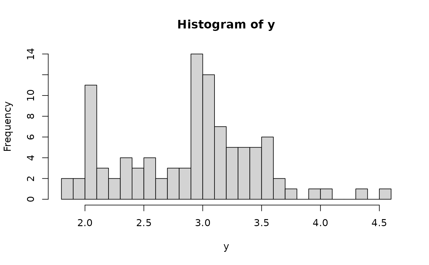
# Simulate data from a transformed (sparse) linear model:
dat = simulate_tlm(n = 100, p = 15, g_type = 'step')
y = dat$y; X = dat$X # training data
y_test = dat$y_test; X_test = dat$X_test # testing data
hist(y, breaks = 25) # marginal distribution
 # Fit the semiparametric Bayesian linear model with sparsity priors:
fit = sblm_ssvs(y = y, X = X, X_test = X_test)
#> [1] "24 sec remaining"
#> [1] "15 sec remaining"
#> [1] "Total time: 49 seconds"
names(fit) # what is returned
#> [1] "coefficients" "fitted.values" "selected" "pip"
#> [5] "post_theta" "post_gamma" "post_ypred" "post_g"
#> [9] "model" "y" "X" "X_test"
#> [13] "psi" "fixedX" "approx_g" "init_screen"
#> [17] "a_pi" "b_pi"
# Evaluate posterior predictive means and intervals on the testing data:
plot_pptest(fit$post_ypred, y_test,
alpha_level = 0.10) # coverage should be about 90%
# Fit the semiparametric Bayesian linear model with sparsity priors:
fit = sblm_ssvs(y = y, X = X, X_test = X_test)
#> [1] "24 sec remaining"
#> [1] "15 sec remaining"
#> [1] "Total time: 49 seconds"
names(fit) # what is returned
#> [1] "coefficients" "fitted.values" "selected" "pip"
#> [5] "post_theta" "post_gamma" "post_ypred" "post_g"
#> [9] "model" "y" "X" "X_test"
#> [13] "psi" "fixedX" "approx_g" "init_screen"
#> [17] "a_pi" "b_pi"
# Evaluate posterior predictive means and intervals on the testing data:
plot_pptest(fit$post_ypred, y_test,
alpha_level = 0.10) # coverage should be about 90%
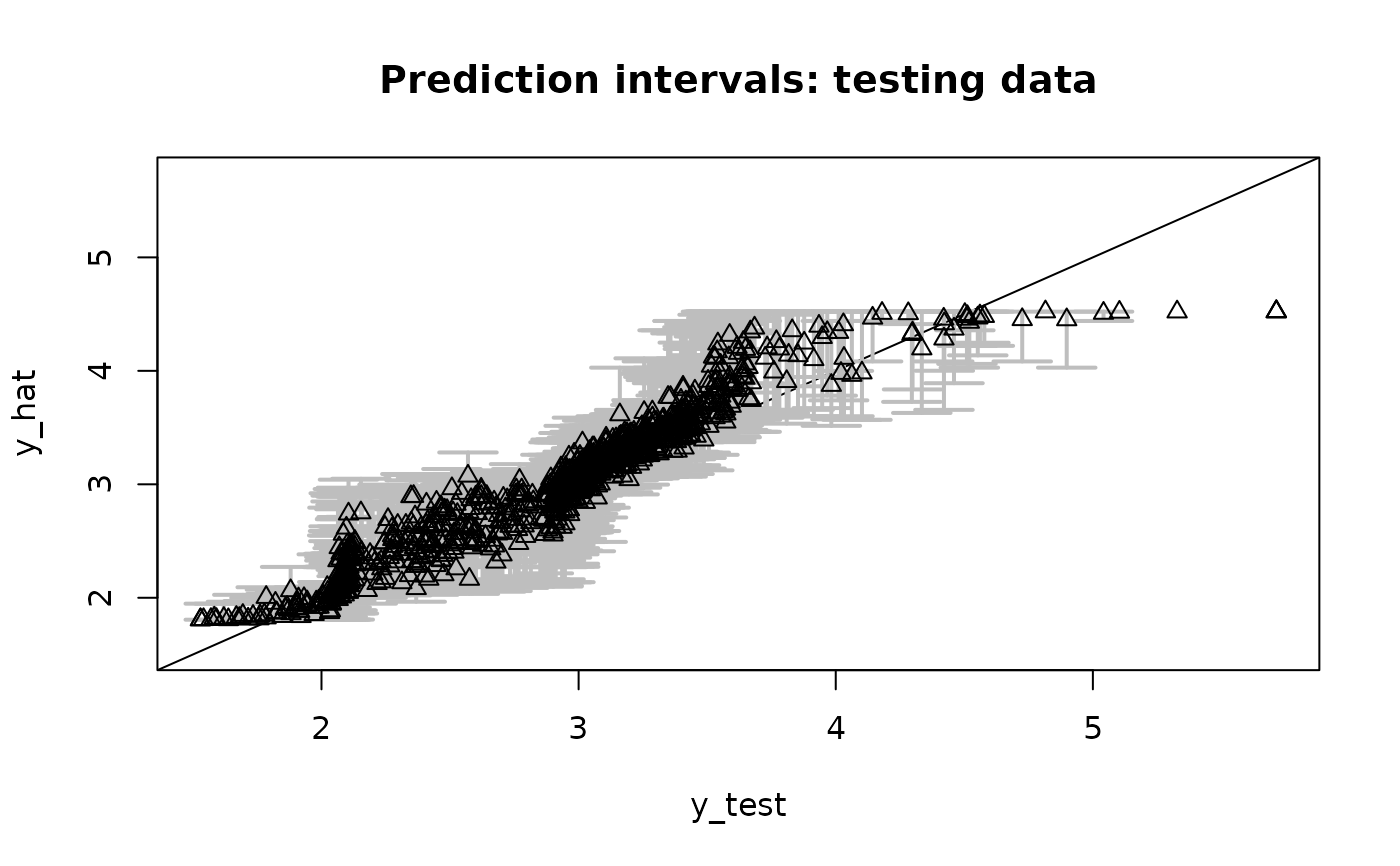 #> [1] 0.937
# Check: correlation with true coefficients
cor(dat$beta_true, coef(fit))
#> [1] 0.9438412
# Selected coefficients under median probability model:
fit$selected
#> [1] 1 2 3 4 5 6 7 8
# True signals:
which(dat$beta_true != 0)
#> [1] 1 2 3 4 5 6 7 8
# Summarize the transformation:
y0 = sort(unique(y)) # posterior draws of g are evaluated at the unique y observations
plot(y0, fit$post_g[1,], type='n', ylim = range(fit$post_g),
xlab = 'y', ylab = 'g(y)', main = "Posterior draws of the transformation")
temp = sapply(1:nrow(fit$post_g), function(s)
lines(y0, fit$post_g[s,], col='gray')) # posterior draws
lines(y0, colMeans(fit$post_g), lwd = 3) # posterior mean
lines(y, dat$g_true, type='p', pch=2) # true transformation
#> [1] 0.937
# Check: correlation with true coefficients
cor(dat$beta_true, coef(fit))
#> [1] 0.9438412
# Selected coefficients under median probability model:
fit$selected
#> [1] 1 2 3 4 5 6 7 8
# True signals:
which(dat$beta_true != 0)
#> [1] 1 2 3 4 5 6 7 8
# Summarize the transformation:
y0 = sort(unique(y)) # posterior draws of g are evaluated at the unique y observations
plot(y0, fit$post_g[1,], type='n', ylim = range(fit$post_g),
xlab = 'y', ylab = 'g(y)', main = "Posterior draws of the transformation")
temp = sapply(1:nrow(fit$post_g), function(s)
lines(y0, fit$post_g[s,], col='gray')) # posterior draws
lines(y0, colMeans(fit$post_g), lwd = 3) # posterior mean
lines(y, dat$g_true, type='p', pch=2) # true transformation
 # Posterior predictive checks on testing data: empirical CDF
y0 = sort(unique(y_test))
plot(y0, y0, type='n', ylim = c(0,1),
xlab='y', ylab='F_y', main = 'Posterior predictive ECDF')
temp = sapply(1:nrow(fit$post_ypred), function(s)
lines(y0, ecdf(fit$post_ypred[s,])(y0), # ECDF of posterior predictive draws
col='gray', type ='s'))
lines(y0, ecdf(y_test)(y0), # ECDF of testing data
col='black', type = 's', lwd = 3)
# Posterior predictive checks on testing data: empirical CDF
y0 = sort(unique(y_test))
plot(y0, y0, type='n', ylim = c(0,1),
xlab='y', ylab='F_y', main = 'Posterior predictive ECDF')
temp = sapply(1:nrow(fit$post_ypred), function(s)
lines(y0, ecdf(fit$post_ypred[s,])(y0), # ECDF of posterior predictive draws
col='gray', type ='s'))
lines(y0, ecdf(y_test)(y0), # ECDF of testing data
col='black', type = 's', lwd = 3)
 # }
# }