Semiparametric Bayesian linear model with horseshoe priors for high-dimensional data
Source:R/source_varsel.R
sblm_hs.RdMCMC sampling for semiparametric Bayesian linear regression with
1) an unknown (nonparametric) transformation and 2) a horseshoe prior for
the (possibly high-dimensional) regression coefficients. Here, unlike sblm,
Gibbs sampling is needed for the regression coefficients and the horseshoe
prior variance components. The transformation g is still sampled
unconditionally on the regression coefficients, which provides a more
efficient blocking within the Gibbs sampler.
Usage
sblm_hs(
  y,
  X,
  X_test = X,
  fixedX = (length(y) >= 500),
  approx_g = FALSE,
  init_screen = NULL,
  pilot_hs = FALSE,
  nsave = 1000,
  nburn = 1000,
  ngrid = 100,
  verbose = TRUE
)
Arguments
- y
n x 1response vector- X
n x pmatrix of predictors (no intercept)- X_test
n_test x pmatrix of predictors for test data; default is the observed covariatesX- fixedX
logical; if TRUE, treat the design as fixed (non-random) when sampling the transformation; otherwise treat covariates as random with an unknown distribution
- approx_g
logical; if TRUE, apply large-sample approximation for the transformation
- init_screen
for the initial approximation, number of covariates to pre-screen (necessary when
p > n); if NULL, usen/log(n)- pilot_hs
logical; if TRUE, use a short pilot run with a horseshoe prior to estimate the marginal CDF of the latent z (otherwise, use a sparse Laplace approximation)
- nsave
number of MCMC simulations to save
- nburn
number of MCMC iterations to discard
- ngrid
number of grid points for inverse approximations
- verbose
logical; if TRUE, print time remaining
Value
a list with the following elements:
coefficientsthe posterior mean of the regression coefficientsfitted.valuesthe posterior predictive mean at the test pointsX_testpost_theta:nsave x psamples from the posterior distribution of the regression coefficientspost_ypred:nsave x n_testsamples from the posterior predictive distribution at test pointsX_testpost_g:nsaveposterior samples of the transformation evaluated at the uniqueyvaluesmodel: the model fit (here,sblm_hs)
as well as the arguments passed in.
Details
This function provides fully Bayesian inference for a
transformed linear model with horseshoe priors using efficiently-blocked Gibbs sampling.
The transformation is modeled as unknown and learned jointly
with the regression coefficients (unless approx_g = TRUE, which then uses
a point approximation). This model applies for real-valued data, positive data, and
compactly-supported data (the support is automatically deduced from the observed y values).
The horseshoe prior is especially useful for high-dimensional settings with
many (possibly correlated) covariates. Compared to sparse or spike-and-slab
alternatives (see sblm_ssvs), the horseshoe prior
delivers more scalable computing in p. This function
uses a fast Cholesky-forward/backward sampler when p < n
and the Bhattacharya et al. (<https://doi.org/10.1093/biomet/asw042>) sampler
when p > n. Thus, the sampler can scale linear in n
(for fixed/small p) or linear in p (for fixed/small n).
Empirically, the horseshoe prior performs best under sparse regimes,
i.e., when the number of true signals (nonzero regression coefficients)
is a small fraction of the total number of variables.
To learn the transformation, SeBR infers the marginal CDF
of the latent data model Fz by integrating over the covariates
X and the coefficients theta. When fixedX = TRUE, the
X averaging is empirical; otherwise it uses the Bayesian bootstrap (bb).
By default, fixedX is set to FALSE for smaller datasets (n < 500)
and TRUE for larger datasets. When pilot_hs = TRUE,
the algorithm fits an initial linear regression model
with a horseshoe prior (blm_bc_hs) to transformed data
(under a preliminary point estimate of the transformation) and
uses that posterior distribution to integrate over theta.
Otherwise, this marginalization is done using a sparse Laplace approximation
for speed and simplicity.
Note
The location (intercept) and scale (sigma_epsilon) are
not identified, so any intercepts in X and X_test will
be removed. The model-fitting *does* include an internal location-scale
adjustment, but the function only outputs inferential summaries for the
identifiable parameters.
Examples
# \donttest{
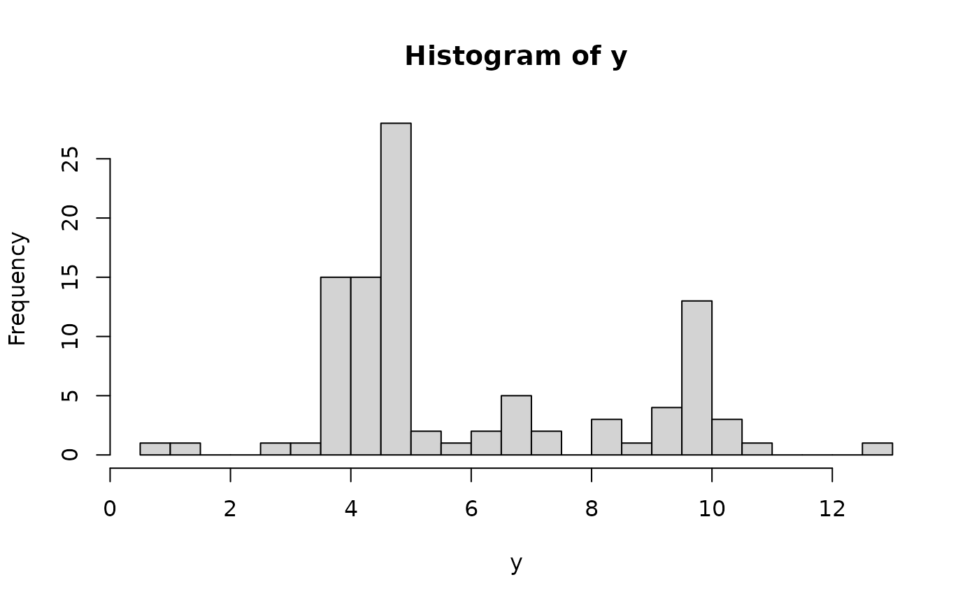
# Simulate data from a transformed (sparse) linear model:
dat = simulate_tlm(n = 100, p = 50, g_type = 'step', prop_sig = 0.1)
y = dat$y; X = dat$X # training data
y_test = dat$y_test; X_test = dat$X_test # testing data
hist(y, breaks = 25) # marginal distribution
 # Fit the semiparametric Bayesian linear model with a horseshoe prior:
fit = sblm_hs(y = y, X = X, X_test = X_test)
#> [1] "3 sec remaining"
#> [1] "3 sec remaining"
#> [1] "Total time: 9 seconds"
names(fit) # what is returned
#> [1] "coefficients" "fitted.values" "post_theta" "post_ypred"
#> [5] "post_g" "post_sigma" "model" "y"
#> [9] "X" "X_test" "fixedX" "approx_g"
#> [13] "init_screen" "pilot_hs"
# Evaluate posterior predictive means and intervals on the testing data:
plot_pptest(fit$post_ypred, y_test,
alpha_level = 0.10) # coverage should be about 90%
# Fit the semiparametric Bayesian linear model with a horseshoe prior:
fit = sblm_hs(y = y, X = X, X_test = X_test)
#> [1] "3 sec remaining"
#> [1] "3 sec remaining"
#> [1] "Total time: 9 seconds"
names(fit) # what is returned
#> [1] "coefficients" "fitted.values" "post_theta" "post_ypred"
#> [5] "post_g" "post_sigma" "model" "y"
#> [9] "X" "X_test" "fixedX" "approx_g"
#> [13] "init_screen" "pilot_hs"
# Evaluate posterior predictive means and intervals on the testing data:
plot_pptest(fit$post_ypred, y_test,
alpha_level = 0.10) # coverage should be about 90%
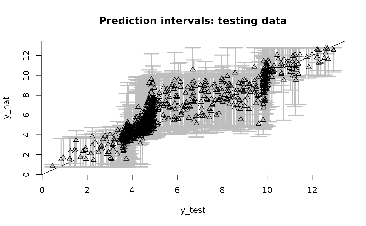 #> [1] 0.835
# Check: correlation with true coefficients
cor(dat$beta_true, coef(fit))
#> [1] 0.9843632
# Compute 95% credible intervals for the coefficients:
ci_theta = t(apply(fit$post_theta, 2, quantile, c(0.05/2, 1 - 0.05/2)))
# True positive/negative rates for "selected" coefficients:
selected = ((ci_theta[,1] >0 | ci_theta[,2] < 0)) # intervals exclude zero
sigs_true = dat$beta_true != 0 # true signals
(TPR = sum(selected & sigs_true)/sum(sigs_true))
#> [1] 1
(TNR = sum(!selected & !sigs_true)/sum(!sigs_true))
#> [1] 1
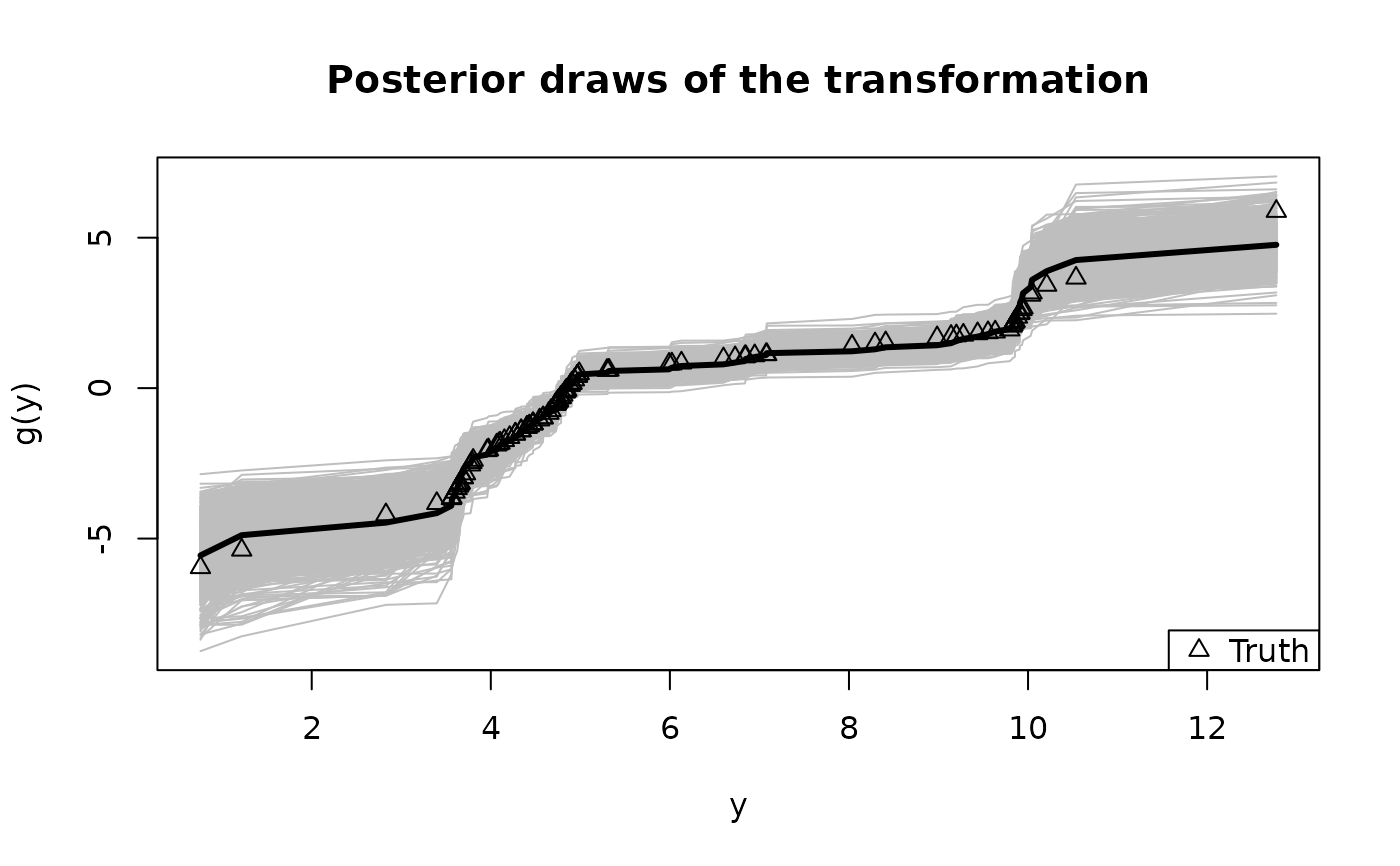
# Summarize the transformation:
y0 = sort(unique(y)) # posterior draws of g are evaluated at the unique y observations
plot(y0, fit$post_g[1,], type='n', ylim = range(fit$post_g),
xlab = 'y', ylab = 'g(y)', main = "Posterior draws of the transformation")
temp = sapply(1:nrow(fit$post_g), function(s)
lines(y0, fit$post_g[s,], col='gray')) # posterior draws
lines(y0, colMeans(fit$post_g), lwd = 3) # posterior mean
lines(y, dat$g_true, type='p', pch=2) # true transformation
legend('bottomright', c('Truth'), pch = 2) # annotate the true transformation
#> [1] 0.835
# Check: correlation with true coefficients
cor(dat$beta_true, coef(fit))
#> [1] 0.9843632
# Compute 95% credible intervals for the coefficients:
ci_theta = t(apply(fit$post_theta, 2, quantile, c(0.05/2, 1 - 0.05/2)))
# True positive/negative rates for "selected" coefficients:
selected = ((ci_theta[,1] >0 | ci_theta[,2] < 0)) # intervals exclude zero
sigs_true = dat$beta_true != 0 # true signals
(TPR = sum(selected & sigs_true)/sum(sigs_true))
#> [1] 1
(TNR = sum(!selected & !sigs_true)/sum(!sigs_true))
#> [1] 1
# Summarize the transformation:
y0 = sort(unique(y)) # posterior draws of g are evaluated at the unique y observations
plot(y0, fit$post_g[1,], type='n', ylim = range(fit$post_g),
xlab = 'y', ylab = 'g(y)', main = "Posterior draws of the transformation")
temp = sapply(1:nrow(fit$post_g), function(s)
lines(y0, fit$post_g[s,], col='gray')) # posterior draws
lines(y0, colMeans(fit$post_g), lwd = 3) # posterior mean
lines(y, dat$g_true, type='p', pch=2) # true transformation
legend('bottomright', c('Truth'), pch = 2) # annotate the true transformation
 # Posterior predictive checks on testing data: empirical CDF
y0 = sort(unique(y_test))
plot(y0, y0, type='n', ylim = c(0,1),
xlab='y', ylab='F_y', main = 'Posterior predictive ECDF')
temp = sapply(1:nrow(fit$post_ypred), function(s)
lines(y0, ecdf(fit$post_ypred[s,])(y0), # ECDF of posterior predictive draws
col='gray', type ='s'))
lines(y0, ecdf(y_test)(y0), # ECDF of testing data
col='black', type = 's', lwd = 3)
# Posterior predictive checks on testing data: empirical CDF
y0 = sort(unique(y_test))
plot(y0, y0, type='n', ylim = c(0,1),
xlab='y', ylab='F_y', main = 'Posterior predictive ECDF')
temp = sapply(1:nrow(fit$post_ypred), function(s)
lines(y0, ecdf(fit$post_ypred[s,])(y0), # ECDF of posterior predictive draws
col='gray', type ='s'))
lines(y0, ecdf(y_test)(y0), # ECDF of testing data
col='black', type = 's', lwd = 3)
 # }
# }